During the past week we have had interesting discussions on this blog about a new paper that tries to filter the AMO signal out of the global temperature series. Several commenters thought that the paper contained serious flaws. Among them was Guido van der Werf, who is a scientist working at the Free University in Amsterdam. His research mainly focuses on forest fires and the effects they have on the carbon cycle. Guido is a friend and I greatly appreciate his efforts to replicate the results of the Zhou/Tung paper. He presents his finding in this guest post.
Guest post by Guido van der Werf
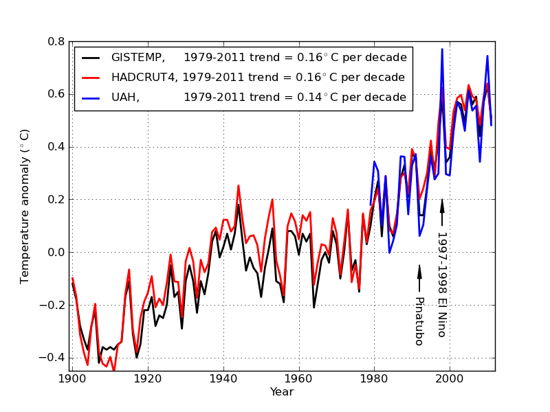
In a recent post Marcel Crok highlighted a new paper by Jiansong Zhou and Ka-Kit Tung in the Journal of the Atmospheric Sciences which halved recent anthropogenic warming and indicated no acceleration of anthropogenic warming over the past 100 years. If true, this is obviously a very important finding. The paper followed on two other papers by Lean and Rind (2008) and Foster and Rahmstorf (2011) aiming to disentangle anthropogenic and natural influences seen in the instrumental temperature record. Three different datasets of temperature are shown below.
To me, studies using the temperature record to study the relative importance of natural and anthropogenic factors are very interesting, for a part because they can be easily repeated and are based on the best data we have. The disadvantage is that they describe what happened in the past, and although this yields information to what may happen in the future it is not a substitute for climate models.
Just a little bit of background information: climate is obviously impacted by a large number of forcings occurring on different time scales. These are both anthropogenic and natural. For example, after the eruption of Mt.Pinatubo in the Philippines in 1991 the global temperature dropped for 2-3 years. And the year 1998 was much warmer than previous and following years because of a strong El Niño episode in 1997-1998. These two events are pointed out in the temperature graph above.
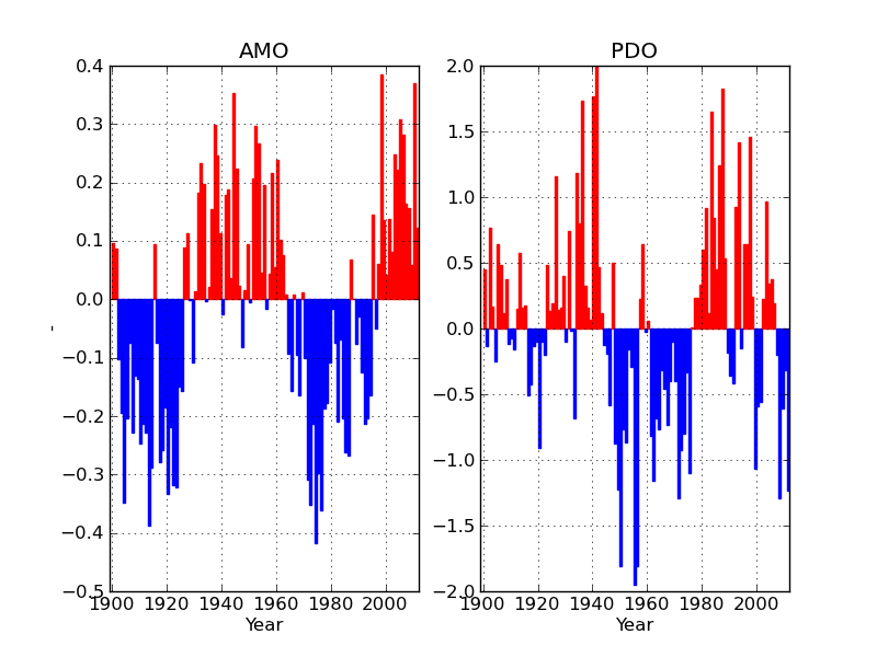
Over decadal time scales things become more complicated. There are at least two ocean oscillations that may impact climate on these time scales: the Pacific Decacal Oscillation (PDO) and the Atlantic Multidecadal Oscillation (AMO), plotted below with positive phases leading to warming and shown in red.
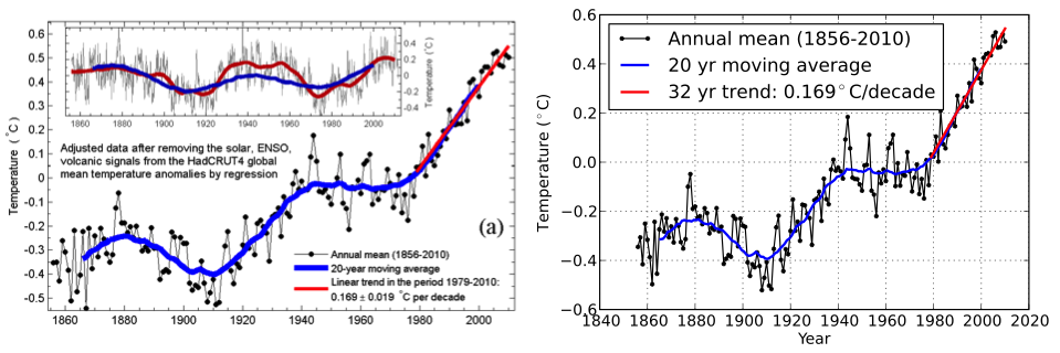
Now, what Zhou and Tung tried to do is subtract the influence of natural variations (AMO, sun, volcanoes, and the El Niño – southern oscillation or ENSO). In theory, what is left behind is the anthropogenic signal. The tool to do this is multiple linear regression (MLR), which basically gives a certain weight to each variable to best match the temperature record. Thanks to the well written paper I was able to reconstruct their results shown in their Figure 1a:
Original and replicated Figure 1a of Zhou and Tong showing the temperature record after the effect of the sun, volcanoes, and ENSO have been subtracted which yields a smoother curve than the “raw” temperature. It shows that there is still a cycle present which looks very similar to AMO. The novelty of the Zhou and Tung study over earlier studies is in that they tried to compensate for this. Basically you add AMO to the statistical method to filter out the natural signals. I was not able to fully replicate their data but came close:
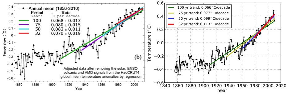
Original and replicated Figure 1b of Zhou and Tong. The temperature record after the effect of the sun, volcanoes, ENSO, and AMO have been taken out. Suddenly the oscillation seen in Figure 1a is gone, and the trend is smaller. In my data I do find a small acceleration which was not seen in Zhou and Tung but the differences are small and may be due to their smoothing of the AMO data, but I am not sure.
To make these graphs they made one crucial assumption. Since none of the natural forcings or oscillation has a trend that can explain the temperature record one has to predefine the shape of the anthropogenic influence over time to be included in the MLR. Lean and Rind (2008) used the net effect of greenhouse gases (warming), changes in albedo (cooling), and aerosols (cooling) for this. Forster and Rahmstorf (2011) used a linear trend, but their study covered only the 1979 onwards period because they included the satellite temperature records which are only available since 1979. For that period the net effect may be rather linear, at least according to the data used by Lean and Rind (2008).
Zhou and Tong used a linear trend as well, but over the much longer time period. So basically they assumed that anthropogenic climate change in 1856 was of the same order of magnitude as in 2011. Below I will repeat their analysis but instead of a linear trend I use the time-evolution of the CO2 concentration, neglecting other greenhouse gases and aerosols which to some degree level out.
Original and replicated Figure 1b of Zhou and Tong with a pre-defined shape of CO2 concentration for the anthropogenic influence in the replicated data instead of a linear trend. The correlation coefficient between modeled and measured temperature is 0.95.
The difference with Zhou and Tong is clear: the acceleration of anthropogenic warming is stronger. Interesting is that in both approaches indicate no halting of anthropogenic warming after 2000; the prevalence of La Nina’s cancel out the anthropogenic forcing.
1940-1970 standstill
What is even more interesting is that the 32 and 50 year trend is still substantially lower than reported earlier. In other words, according to this simple analysis part of the 1970-2000 warming was due to the upswing of AMO. Similarly, the 1940-1970 flat temperature may have been the result of the downswing of AMO canceling the greenhouse gas warming. This provides in my opinion a more elegant explanation than the aerosol explanation most commonly used, but more research is needed to better pinpoint whether this is true.
If we were to convert the CO2 concentration to radiative forcing (RF) using the well established formula RF = 5.35 * ln(CO2 / CO2pre-industrial) and put this in the MLR, the slope for RF is 0.42 degree C warming per unit W/m2. A doubling of CO2 is 3.7 W / m2 so combining these numbers yields a transient climate sensitivity of 0.42 * 3.7 = ±1.5 degrees C. Clearly, these are not much more than back of the envelope calculations but still valuable.
Summarizing:
- It is important to include AMO in any regression analysis to deduce the warming trend as shown by Zhou and Tung
- The outcome of this exercise is highly dependent on the assumed shape of the anthropogenic signal. If we assume that the anthropogenic influence is not linear then anthropogenic warming is accelerating
- The climate sensitivity of the system seems lower than the usually assumed values, although this also depends on the time period covered in the MLR
- Anthropogenic warming has not stopped in 2000 or so, this result is independent of the assumption on the shape of the anthropogenic influence in the MLR
Major uncertainties in this approach are related to:
- The temperature record, which is in the 19th and first part of the 20th century based on a limited number of stations
- The anthropogenic influence on AMO; we simply used the detrended values but accounting more precisely for the anthropogenic impact may give different results
- And of course the shape of the anthropogenic influence. A linear influence seems unjustified, but the CO2 concentration as a proxy as I did is not perfect either
- For the calculation of the transient climate sensitivity the relative role and time evolution of other greenhouse gases than CO2 and aerosols is crucial.
- And anything else I overlooked, please respond!


Hello Guido, Very nice investigation of the Zhou-Tung article. I didn’t do the mathematics or read their paper (paywall), so I take your word for it that they used a linear anthropogenic trend from 1856. That would be rather silly. I think you jump to conclusions in stating that the AMO is a better explanation for the 1945-1970 standstill than aerosols are. Humanity has produced a lot of sulfur dioxide the last century which increased quickly after WW2. See for instance figure 3a in http://www.atmos-chem-phys.net/11/1101/2011/acp-11-1101-2011.pdf Physics tells us that aerosols do have an influence on incoming solar light (Mie scattering)… Lees verder »
Thanks Jos – good suggestions, I will try to include them in a follow-up or report on the findings here. The SO2 emissions are interesting, and I can understand they played a role in the flat temperature. On the other hand, emissions decreased over 1975-2000, this may thus also explain part of the temperature rise over that period.
Thanks also for finding the mistake in the temperature graph, I made the mistake of using temperature over land only. The graph is corrected now.
Guido can you show the residual after subtracting the co2 forcing using a sensitivity of 1.5 degrees C per doubling?
Marcel, it is quite well known that aerosols are the predominant cause of the mid 20th century cooling (nb: I’m not saying it is the ONLY reason). The statement that the AMO natural variability is a more elegant explanation is quite outrageous, and though you personally might like it, it is certainly not backed up by the current state of knowledge of the climate system!
[MC: Arjan, this is a guest post written by Guido van der Werf.]
Arjan it is quite well known that aerosols are the fudge factor in the climatemodels. High CO2 sensitivity models have strong aerosol cooling and low CO2 sensitivity models have weak aerosol cooling.
Hans – will do tomorrow, good suggestion, thanks. Arjan – you may be right, but I know of at least a few climate scientists that are not fully comfortable with the aerosol explanation. I agree with you that it has contributed, but how much is not resolved I would say. And again, if aerosols have contributed to the standstill then the aerosol decrease has also contributed to the 1970-2000 warming. Probably a more detailed look into the different hemispheres and land versus ocean may help disentangling the effects. I will dig up some literature but if you have good suggestions… Lees verder »
Guido, have a look at this picture regarding the period 1998-2011:
http://www.knmi.nl/cms/viewimage.jsp?number=109830
The cooling due to El Nino/La Nina since 1998 is quite clear, also the cooling around Antarctica and the seas in the east part of Azia. The Arctic has warmed a lot in this period, which is an understatement.
Full text at:
http://www.knmi.nl/cms/content/68206/stijging_wereldgemiddelde_temperatuur
And of course has the decrease in aerosols contributed to the 1970-2000 warming, e.g. the US Clean Air Act started in 1963 and was expanded in 1967:
http://en.wikipedia.org/wiki/Clean_Air_Act_%28United_States%29
Hans, please see here for a plot with data and MLR model as well as residuals. Based on the CO2 concentration as a proxy for anthropogenic influence instead of a linear trend.
Guido, Thank you very much for this re-analysis of the Zhou and Tung paper ! That’s great work, and I admire you for spending the time to replicate their results. I argued that their resulting trend is artificially created, because of the AMO index they used. They regressed the AMO index out of the global temperature record, but since the AMO index mostly consists of the global temperature signal itself, they ended up with the linear trend that is subtracted from the AMO index by definition. Since Zhou and Tung’s is allegedly a result of their own method, I don’t… Lees verder »
Sorry, Guido, I take my speculations about the equilibrium formula back.
In fact, I don’t know where you obtained that formula. Can you tell us ? and also why you think it applies for the increase in CO2 over the past couple of decades ?
@Hans Erren: There is a large uncertainty in the aerosol forcing and its coupling with the hydrological cycle. It is terribly frustrating (and maybe also quite bad for our future) that though we have tremendously improved our knowledge on both in the last 30 years, we do not seem to be able to significantly reduce the uncertainties in the climate effects of both. Just adding more details does not seem to work (yet..). The last 150 years of surface measurements are not a good constraint for climate sensitivity to greenhouse gas forcing. In general, on the extreme sides of the… Lees verder »
I would have no problem with this type of regression analysis if it were presented as a “what if” exercise (as check of consistency of certain assumptions with the data) but it proves nothing and you can’t attach much meaning to it. It’s a kind of game. In particular the interpretation of the regression on a linear trend or CO2 concentration (the log of which is almost linear) as “anthropogenic” is pure speculation (Would there be no long term trend without human effects? That is a strong assumption. All we know is that climate fluctuates on a wide range of… Lees verder »
@Guido I tried to reproduce your results using multiple regression on HadCRUT4 year-average temperatures against TSI, Stratospheric Aerosols, Nino3.4, LN(CO2) and AMO/PDO/non-ghg-human forcings(Giss), but ended up with quite different numbers. I got the following trends for the human part of global warming signal from 1970 to 2010, in °C/decade: without AMO: 0.166 with AMO: 0.141 with Aerosol-Forcings: 0.162 with AMO and Aerosol-Forcings: 0.134 Some of the difference could be due to the fact that I started with the regression in 1900, to leave out the period with the largest uncertainty in the data. Did you use the standard AMO index?… Lees verder »
@Guido
Be aware that global population correlates 99% with CO2, and that e.g. UHI is proportional to log(pop). Statistically it is therefore impossible to make a distinction between effects that are related to log(pop) and log(co2)
http://members.casema.nl/errenwijlens/co2/pop1gvsco2.gif
Guido, You mention : Below I will repeat their analysis but instead of a linear trend I use the time-evolution of the CO2 concentration, The more I look at that result (last 30 year trend 0.113 C/decade) the more confused I get as to how you obtained that number. All of the prior studies (Lean and Rind (2008), Forster and Rahmstorf (2011) and even the study you are commenting on Zhou and Tung (2012)) start from the global temperature record, and they try to eliminate natural forcings (volcanoes, ENSO, solar activity etc). Basically, they try to obtain the temperature trends… Lees verder »
Going through the discussion from top to bottom: @Rob Dekker: for the conversion from CO2 concentration to radiative forcing please see for example the IPCC which is partly based on the work of Myhre et al. (1998) @Cees de Valk: in essence it is a what-if study. It is a poor-man’s version of a more complicated physical model I would say. What this blog and also Jos’ results below show that one has to be very careful with the assumptions that go into the regression. I disagree with the linear trend as used by Zhou and Tung, but I am… Lees verder »
@ Guido
I was thinking of the repeated warnings by Roger Pielke Sr. that land use change is underexposed in climate models, and landuse change is proportional to popoulation growth. So if you find purely by correlation that CO2 has a sensitivity of 1.5 without taking land use into the equation, then you overestimate climate sensitivity. By how much is extremely difficult to establish, given the 99% correlation between CO2 and population.
http://pielkeclimatesci.wordpress.com/2012/10/11/the-importance-of-land-useland-cover-as-a-first-order-climate-forcing/
Hans – I see, thanks for explaining. I have spend quite a bit of time looking at albedo changes due to land use change, and it is a factor that can more important for regional climate than higher GHG concentrations. On a global scale I don’t think there is a lot of evidence that it a major player though. My thinking of choosing CO2 concentration is that the other positive forcings (CH4, N20, O3, halocarbons) would cancel out of some of the negative forcings (aerosols, albedo). According to the IPCC they do on a global scale. But as you and… Lees verder »
@Guido, thanks very much for your response. Just to clear up a few things: You wrote “I disagree with the linear trend as used by Zhou and Tung, but I am also aware that the CO2 proxy I used isn’t perfect either”. Now, CO2 may be a better representation of something proportional to the anthropogenic contribution to radiative imbalance (its log would be better though, and if sensitivity would be high, you would expect a significant lag due to ocean warming etc), but the OUTCOME of your regression does not (and cannot claim to) distinguish a CO2 effect from e.g.… Lees verder »
@Guido I repeated my analysis with the NOAA AMO data you used in your analysis and I get the same result as you do: 0.112 °C/decade for 1970-2010. This drops a little to 0.109 °C/decade when I add the Giss non-natural forcings without ghg’s (= aerosol effect + land-use change + black carbon + tropospheric ozone). Looking at your results and mine, your assumption that CO2 and the other human induced forcings (e.g. aerosols) almost cancel each other out is quite reasonable. I would not calculate any climate sensitivity from such a regression analysis, because it is unclear if the… Lees verder »
Jos Hagelaars said your assumption that CO2 and the other human induced forcings (e.g. aerosols) almost cancel each other out is quite reasonable That’s not really what Guido is saying. He states : neglecting other greenhouse gases and aerosols which to some degree level out. I think that Guido is correct on this. Other (not CO2) greenhouse gases (Methane and other halocarbons, ozone, etc) may indeed level out with aerosols to some extent : http://en.wikipedia.org/w/index.php?title=File:Radiative-forcings.svg&page=1 But it’s very clear that CO2 is the dominant greenhouse gas which does not “cancel out” other human induced forcings. I assume your statement was… Lees verder »
Guido said I did the analysis in Python and will post the code and the array of input data tomorrow on my website so you can have a look at it Looking forward to that Python code, Guido. But, before we start debugging your code, it would be nice to understand what it is supposed to do. Since you are a scientist, could you please explain how you introduced the “pre-defined shape of CO2 concentration for the anthropogenic influence” into the multiple linear regressions ? In other words : what exact have you done to produce your last figure (which… Lees verder »
@Rob Dekker,
You are absolutely right, I certainly did not mean that the effects of CO2 and aerosols cancel out.
I noticed with these regression analysis that when you add the forcings of the other GHG’s + [all the other non-natural/non-GHG] forcings (e.g. aerosols) the result is about the same as when you use only LN(CO2). Which is about the same as the IPCC picture says and what Guido said.
Sorry about the confusion, my English needs to be improved a lot.
@Rob Dekker – please see here for the python code I used to get Figure 1a and 1b. To get the last graph just toggle lines 129 and 130. I found another mistake which underestimated the transient climate sensitivity, it now changed from 0.41 to 0.50 for dt / dRF (or, 1.8 degrees per doubling, transient). I will start exploring other AMO datasets when I find some time, thanks for the suggestions. @Cees de Valk – you are totally right, if one would build in a lot of delays in the system and non-linearities one could probably match the temperature… Lees verder »
Guido, Thanks for your Python code. It clarifies a lot. In fact, it confirms my concerns with the method you use, and explains why you are getting a lower ‘anthropogenic’ trend than Lean and Rind (2008) and Foster and Rahmstorf (2011) for the past 30 years. The problem, as it was in Zhou and Tung, is again (extreme) ‘contamination’ of the variables in MLR. Here is the problem : You did NOT change the AMO definition. You still use Zhou and Tung’s flawed definition which is heavily contaminated by (correlated with) the global temperature record). So, the entire global temperature… Lees verder »
@Guido: So you want to bet! I like betting. But only on verifiable future outcomes, not on an explanation for something. For the explanation of global average temperature, I prefer http://www.venganza.org/about/open-letter/. Solid statistical analysis with carefully motivated choice of explanatory variables. More evidence: the number pirates seems somewhat on the increase again, and guess what happened recently?
@Rob Dekker, let’s recap: – The 1979-2010 trend in the temperature datasets: 0.16 degrees per decade – Foster and Rahmstorf say this is an underestimate because in the latter part of the record natural fluctuations lower the trend, the anthropogenic trend should be 0.18 degrees per decade – Zhou and Tung used the AMO as an additional natural fluctuation, focus on a much longer timeframe, and find 0.07 degrees per decade – I think that was due to at least one flawed assumption and repeated the analysis with a more sensible (but not perfect) assumption, boosting it again to 0.11… Lees verder »
@Cees de Valk: apologies, that was not an honest bet, here we go again without the special characters: Temperature over 2011-2020 minus 2001-2010 above 0.10 degrees C: you give me 100 euro to be donated to charity (my choice) Temperature over 2011-2020 minus 2001-2010 below 0.05 degrees C: I give you 100 euro to be donated to charity (your choice) In between: we go drink a beer and discuss the current state of climate science Temperature based on average of most recent versions of GISS, UAH, HADCRUT. How about that? Now, the Bounty unfortunately sank so keep in mind we… Lees verder »
A bit late, but think this is a nice example of how a blog discussion can help in writing a scientific paper: the comments of everyone above have helped me in improving a paper that is now published in Earth System Dynamics. Thanks!
Congratulations Guido and wellcome back from Indonesia!
Marcel
The big upsurge in industrial production after World War Two was almost entirely in the older industrial countries- North America, Western Europe and (to a lesser extent) the Communist countries. Industrial production outside these areas began to take off in the late 1950 (the four small ASsian “tigers”) and really got under way during the 1970s and 1980s- India, China and many others.Aerosols (sulfide dioxide and particulates), visible in clouds and smog, certainly increased after 1945. until air pollution policies began to be implemented in the late 1950s (Britain 1956). If these were the cause of falling temperatures- offsetting, so… Lees verder »